Shazam finds songs by voting on time offsets, not by comparing audio

Point a phone at a ceiling speaker in a loud cafe and Shazam names the track in about a second, from a catalogue north of a hundred million songs, off five seconds of audio that also contains an espresso machine and two conversations. The interesting part is not that this works. It is that it works without ever comparing audio to audio.

Everything public about the mechanism comes from one paper: Avery Wang’s “An Industrial-Strength Audio Search Algorithm” (2003), written by Shazam’s co-founder. This log follows that paper. Where the paper stops, I say so, because Shazam has been inside Apple since 2018 and the production stack since then is not public.

Why similarity search is dead on arrival

The naive design is a nearest-neighbour search: embed the clip, embed every track, find the closest. For this problem it fails twice before it starts.

First, the query is not a degraded copy of the track. It is five seconds out of two hundred, at an unknown position, through a phone microphone, a room, and a lossy codec. Waveforms do not survive that. Even spectrogram distance is fragile, because the noise floor in a cafe recording is a different signal added on top, and distance metrics count all of it.

Second, the latency budget is about a second against a catalogue of hundreds of millions of tracks. Whatever the representation is, the lookup has to behave like a hash table, not like a scan.

So the design inverts the question. Do not ask “which track sounds most like this clip”. Ask “which track contains these exact landmarks, in this exact arrangement”. Exact-match lookups are what databases are good at.

Peaks: what survives a bar at midnight

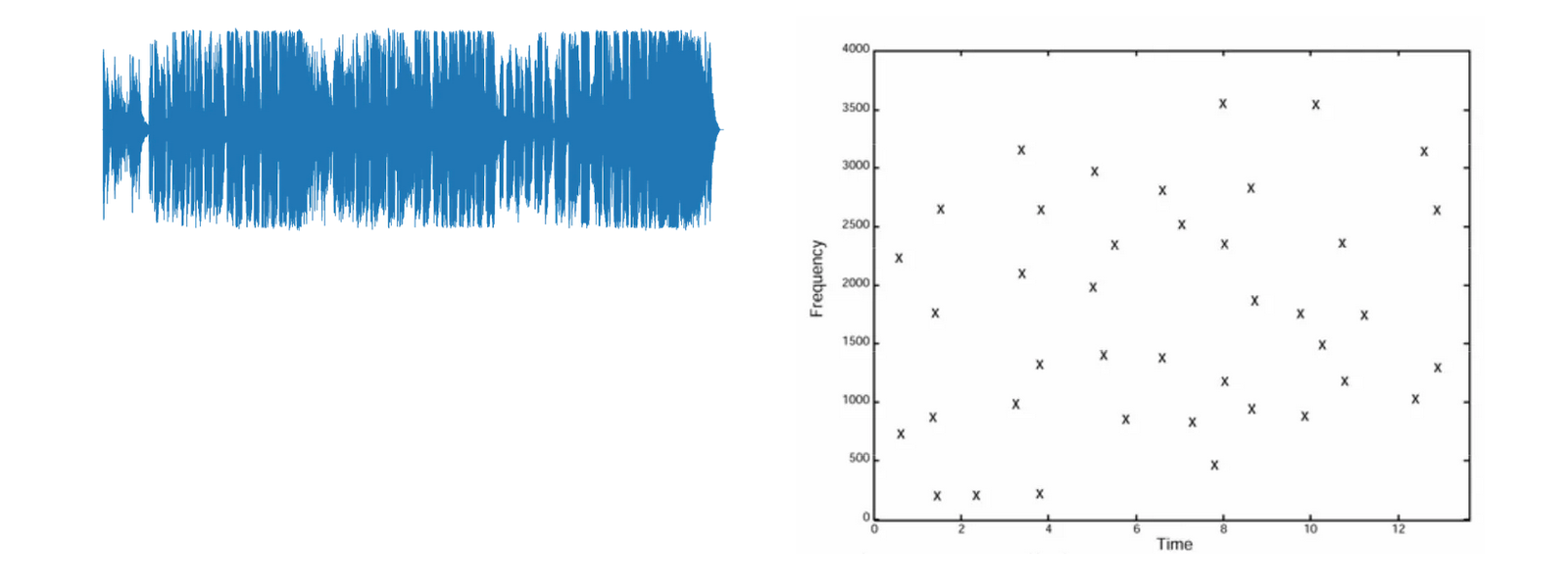
The pipeline starts with a spectrogram, time on one axis, frequency on the other, energy as intensity. Then it throws almost all of it away and keeps only local energy maxima: points that are louder than everything around them in a time-frequency neighbourhood. The paper calls the result a constellation map, because once you discard amplitude and keep only (time, frequency) coordinates, it looks like a star field.

Peaks are the right thing to keep because additive noise raises the floor but rarely dethrones the strongest components. The chatter in a cafe adds energy across the band; the chorus hook is still the loudest thing at its frequency. A recording made through a phone in a noisy room and the studio master produce overlapping constellations, which is the property everything downstream depends on.

Single peaks are not selective enough

Here is the trap I fell into the first time I wrote about this system: treating one peak as one fingerprint. It cannot work, and the reason is entropy.

A peak frequency, quantized for indexing, carries maybe 8 to 10 bits of information. Every track has thousands of peaks. Index single peaks and each lookup key collides with a meaningful fraction of the entire catalogue; the postings list for “something around 1 kHz” is millions of entries long. You have built a hash table where every bucket holds half the database.

The paper’s fix is combinatorial hashing. Take each peak as an anchor. Look ahead into a small target zone and pair the anchor with each of the next few peaks, fan-out factor F of around 10. Each pair becomes a hash of three numbers: anchor frequency, target frequency, and the time gap between them, packed into roughly 32 bits.

def landmark_hash(f_anchor: int, f_target: int, dt: int) -> int:
    # ~10 bits per frequency band, ~12 bits of time delta: one 32-bit key.
    return (f_anchor << 22) | (f_target << 12) | dt

A specific frequency is common. A specific pair of frequencies a specific number of milliseconds apart is rare. Pairing multiplies the number of index entries per track by F, and in exchange each key becomes selective enough that a lookup returns a short postings list. The paper is explicit about this trade: storage grows by the fan-out, search time shrinks combinatorially, because you are matching 30-bit landmarks instead of 10-bit points.

The index itself is the least exotic part. It is an inverted index: hash value maps to a postings list of (track id, anchor time) pairs, precomputed once per track at ingest. The 2003 paper did this with sorted arrays on commodity hardware.

Matching is a histogram, not a search

The query path runs the same pipeline on the sample: spectrogram, peaks, pairs, hashes. Then comes the part that makes the system work, and that most retellings (including my earlier one) leave out entirely.

Each sample hash that hits the index yields candidates: track T contains this landmark at time t_track, and the sample contains it at time t_sample. Compute the offset, t_track minus t_sample. Now group candidates by track and look at the offsets.

If the sample genuinely is 5 seconds of track T starting at 1:32, then every surviving landmark agrees: the offset between its position in the track and its position in the sample is 92 seconds, give or take quantization. Spurious hash collisions from other tracks produce offsets scattered uniformly. So the decision rule is: build a histogram of offsets per candidate track, and declare a match when one bin spikes.

def score(track_offsets: list[int], bin_ms: int = 50) -> int:
    bins: dict[int, int] = {}
    for offset in track_offsets:
        b = offset // bin_ms
        bins[b] = bins.get(b, 0) + 1
    return max(bins.values(), default=0)

graph TD
    A[5s sample] --> B[Spectrogram + peaks]
    B --> C[Pair peaks into hashes]
    C --> D[Inverted index lookup]
    D --> E["Candidates: (track, t_track, t_sample)"]
    E --> F[Offset histogram per track]
    F --> G{One bin spikes?}
    G -->|yes| H[Match: track + position]
    G -->|no| I[No match]

Two properties fall out of this, and they are the ones that feel like magic from the outside.

Noise tolerance is free. Matching does not need most hashes to survive the cafe; it needs enough survivors to stack one histogram bin above the noise floor. The paper reports correct identification with only a small fraction of landmarks intact, which is why a clip that is mostly espresso machine still resolves.

Position comes out as a by-product. The winning offset does not just say “this is Bohemian Rhapsody”, it says where in the track the sample sits. That is how the app can sync lyrics to the recording position without any extra work.

I keep coming back to how cheap the final decision is. After all the signal processing, the match itself is a group-by and a max over small integers. The heavy thinking was moved to ingest time, once per track, so that query time is arithmetic.

The arithmetic at catalogue scale

Illustrative numbers, not Shazam’s: at a peak density around 10 per second and fan-out 10, a 3-minute track yields on the order of 100,000 landmark hashes. A catalogue of 100 million tracks is around 10^13 postings of a few bytes each. That is tens of terabytes: large, but flat, append-mostly, trivially shardable by hash prefix, and every query is a batch of point lookups followed by a histogram. There is no graph to traverse and no model to evaluate on the hot path. Sharding, caching hot tracks, and fanning out lookups are all standard from here; the algorithm did the hard part by making the workload embarrassingly partitionable.

Where the paper stops

The 2003 paper is the last authoritative public description. Since the Apple acquisition, reasonable guesses (on-device fingerprinting for the always-on “auto Shazam” mode, neural embeddings somewhere in the stack) are just that, guesses. Google published a different design for its Now Playing feature built on learned embeddings and vector search, which shows the constellation approach is not the only way to solve this class of problem. What the constellation approach uniquely buys is exact-match index semantics and an interpretable decision rule, which is a lot of operational simplicity for a system that has to answer in a second.

Correction

An earlier version of this log described the fingerprint as a hash of a single peak’s time and frequency concatenated into one integer, matched by array lookup. That was a toy I presented as the real thing, and it is wrong in ways that matter: single peaks are not selective enough to index, hashing absolute time into the key breaks matching at any other position in the track, and without offset voting there is no noise tolerance at all. The version above follows the published algorithm. I would rather carry a visible correction than a clean-looking page that teaches the wrong mechanism.